Retro.Know-How

AmigaOS was an operating system that was way ahead of its time. It had features that other home operating systems (like Windows or MacOS) were missing back then, like preemptive multitasking. There was also a feature that was called assignments. I truly miss that one on Linux!

An Amiga "assign" is a bit similar to the drive letter you may know from Windows. For example, the Windows path C:\example.txt refers to a file called example.txt in the root directory of the main partition, while the same file on the first floppy drive is called A:\example.txt.

On Amiga, the main partition is usually called DH0:, the second partition is called DH1: and so on, while the first floppy drive is called DF0:. A similar path on the Amiga would thus be DH0:example.txt or DF0:example.txt.

As you can see, on the Amiga a "drive letter" can actually consist of multiple characters and also numbers. This is called an assignment. The name DH0 is assigned to the main harddisk partition.

But wait, there is more!

You can have multiple assigns pointing to the same target. For example, the main partition usually contains the Amiga desktop environment, called Workbench. For this reason, the main partition also has a label like Workbench, and the file could also be accessed as Workbench:example.txt.

This is actually quite a smart concept, especially for exchangeable media. For example, let's imagine we have just started a game called shredzone, and it needs to access a file Music/Opening.mod on its installation disk (AmigaOS uses a slash as file separator, like all proper operating systems). It would open a file called shredzone:Music/Opening.mod.

AmigaOS would see that there is no assignment called shredzone, and would pop up a dialog like this:

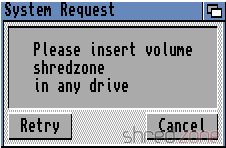
From a user's perspective, I would now know that I have to find a medium called shredzone, and insert it into the computer. It does not matter if it's a floppy disk, a CD, or even a network mount. AmigaOS also does not command me to insert the medium into a certain drive. If it's a floppy disk, and I have multiple floppy drives, I can just pick the one I like to. AmigaOS will then detect that a medium with that name was inserted, would close the dialog, and grant the game access to the file.

On Linux, I would need to access that medium under a path like /run/media/shred/shredzone, which is a lot to type, contains my user name, and is harder to remember than just shredzone:.

But wait, there is still more! 😄

It is easy to add assignments to the system via command line. It's even possible to use subdirectories as assignment target. Let's stay with our shredzone game example. I got tired of having to insert the installation disk every time I want to play that game. So I create a directory called DH2:Games/Shredzone/Files on my hard drive, and I copy all files of that disk to that directory.

After that, I enter this command on the command line:

assign shredzone: DH2:Games/Shredzone/Files

Now, when I start the game, AmigaOS will see that there is a shredzone assign already existing, and will access the files there. So the song file shredzone:Music/Opening.mod would be accessed at DH2:Games/Shredzone/Files/Music/Opening.mod.

AmigaOS makes use of assigns itself. For example, there is a standard assignment called C:. It usually points to the C directory of the booting device, where all command line commands (like dir, copy, delete etc) are expected to be present. This assign is similar to what $PATH is to a Linux shell.

Imagine I have installed a set of development tools, like an assembler and a C compiler. The commands of this toolset can be found at DH1:Development/DevTools/C. On a Linux system, I would add this path to the $PATH env variable, so I can just type the command name to execute one of these commands.

On AmigaOS, I just add this path to an existing assignment:

assign add C: DH1:Development/DevTools/C

Now AmigaOS knows that when I enter a command in the command line, it has to look for it in Workbench:C, and if it's not found there, it will try to find it in DH1:Development/DevTools/C. I could even execute commands like dir C:, and see all files in both directories. Of course, it is not limited to two targets.

There is still more, like deferred assigns. But I only want to give you a general impression of what Amiga assigns are, and why I miss them on Linux.

The one thing computers are really good at is calculating. You might now expect that all CPUs are capable of the four basic arithmetic operations, but that isn't the case. The first 8 bit processors were only able to add and subtract numbers, and even the subtraction was performed by adding the negated subtrahend. Multiplication and division instructions first appeared on 16 bit processors, albeit they were still very slow in the first generation.

Simple multiplications and divisions by powers of two can be achieved by shifting a value bitwise to the left or right, respectively. This is, shifting a value by one bit to the left is the same as multiplying it by 2, while shifting by two bits to the left multiplies it by 4, and so on.

But how can we multiply any two numbers? It has to be done step by step, by using basic operations like addition or bit rotation. This article will explain how it works on a Z80 CPU.

Back at school, we have learned to multiply large numbers by long multiplication. Basically, we break up the problem by multiplying the multiplier with each digit of the multiplicand, and then summing the products. For example, if we want to compute the product of 27 and 12, we compute 27×2 = 54 and 27×1 = 27, and then sum the products 57+270 = 324.

  27 × 12
———————————
       54
 +    27∙
———————————
      324

We can use the same algorithm on a computer. But wait, wouldn't we still have to multiply, even if with smaller numbers? Actually, no! Since computers use binary digits, we only need to multiply either by 1, giving the value itself, or by 0, always giving 0.

This is the the same long multiplication of 27 (11011) and 12 (1100) with binary numbers:

  11011 × 1100
————————————————
         00000
        00000∙
       11011∙∙
 +    11011∙∙∙
————————————————
     101000100

The steps can be executed in a loop. At the beginning, a result register is initialized with zero. If the rightmost bit of the multiplicand is 1, the multiplier is added to the result register. After that, the multiplicand is rotated to the right by one bit, and the multiplier is rotated to the left by one bit. This loop is repeated until the multiplicand is zero, because the result won't change after that anymore.

The following Z80 assembler code example multiplies the values in the BC and DE register pairs, and returns the product in the HL register pair. If an overflow occured during multiplication, the Carry flag will be set.

The multiplicant is kept in the BC register pair. To rotate it one bit to the right, we first use the srl b instruction. It rotates the B register, moving the value of bit 0 to the Carry flag, and inserting a 0 to bit 7, so the multiplicant is filled up with zeros with each rotation. After that, rr c rotates the C register and moves the content of the Carry flag to bit 7. Both instructions combined rotate the BC register pair one bit to the right, insert a 0 to the highest bit. The lowest bit is moved to the Carry flag, where it can be tested.

We essentially do the same with the multiplier in the DE register pair, but in the opposite direction. As a rotation to the left by one bit essentially just doubles the value, we also could have used add de,de. Sadly the Z80 does not offer such an instruction.

multiply:	ld	hl, 0		; clear the result register
.loop:		ld	a, b		; is BC == 0?
		or	c		;   (also resets carry flag)
		ret     z		; then we're done!
		srl	b		; logical right shift of BC
		rr	c		; bit 0 goes to carry flag
		jr	nc, .zerobit	; unless bit 0 was 0
		add	hl, de		; add multiplier to result
		ret	c		;   return on overflow
.zerobit:	sla	e		; shift multiplier to the left
		rl	d		;   topmost bit goes to carry flag
		ret	c		;   return on overflow
		jr	.loop		; next iteration

The example only multiplies positive integers. To multiply negative integers, we first need to change all factors to positive numbers and do the multiplication. The result then needs to be negated if one of the factors was negative, but not both.

While cleaning up the cellar, I found my Amiga 500 and also a GVP Impact Series II SCSI host adapter. Inside, there was a Fujitsu M2611SA harddisk. After about 25 years, I had totally forgotten about it, and I wondered what was stored on it. So let me take you on the adventure trip of how to salvage old Amiga harddisks on modern Linux machines.

The Amiga ecosystem has always been very SCSI friendly. Commodore broke this tradition only with the final AGA models, where they switched to the IDE bus to reduce costs. The Amiga community never approved this change, and many accelerator cards that were sold for these machines also came with a SCSI host adapter. The SCSI bus was a lot faster than the IDE bus. Also a single ribbon cable could connect up to seven SCSI devices, where the IDE bus only permitted two devices.

Today this SCSI affinity turns out to be a problem though. SCSI was never a topic on consumer PCs, so there are no SCSI-to-USB adapters on the market (I wish they were), and SCSI cards for the PCIe bus are very expensive. I'm still having an Adaptec SCSI card in my cupboard that I bought many years ago, but it is for the old-style PCI bus. Luckily there are PCI-to-PCIe adapters available on the market, so I could reuse this old card in my computer. The card stack looks adventurous, but it will do for a few hours of operation to backup the data.

The big question is: Can a modern Linux machine even read Amiga formatted harddisks?

Mounting Amiga Harddisks

Yes, it can. It seems that there are a lot of Amiga fans among the Linux kernel developers. The Amiga uses a different partition table scheme than PCs, but if you're lucky, your Linux will still detect the Amiga partitions and offer them as e.g. /dev/sdg1. Then all you need to do is to mount the partition via mount.

It didn't work on Fedora though, so I had to do some more typing. First I had to find out the offsets of the individual partitions. GNU Parted can be used for that, as it is able to decode Amiga partition tables:

# parted /dev/sdg
GNU Parted 3.3
Using /dev/sdg
Welcome to GNU Parted! Type 'help' to view a list of commands.
(parted) u
Unit?  [compact]? b
(parted) p
Model: FUJITSU M2611S (scsi)
Disk /dev/sdg: 45078528B
Sector size (logical/physical): 512B/512B
Partition Table: amiga
Disk Flags:

Number  Start   End        Size       File system  Name  Flags
 1      52224B  45078015B  45025792B  affs1        DH0   boot

(parted) q

So there is only one partition on the HD. It starts at offset 52224 and is Amiga FFS formatted. Luckily most Linux distributions are able to mount this file system out of the box. The start offset is needed to mount the partition. I also mount it read-only to make sure that I won't accidentally change or delete my precious old data.

mount -o ro,offset=52224 -t affs /dev/sdg /mnt/

Et voilà:

# ll /mnt/
drwx------. 1 root root    0 Apr 16  1997 C
drwx------. 1 root root    0 Jun 11  1994 Devs
-rw-------. 1 root root 1233 Apr 16  1997 Devs.info
drwx------. 1 root root    0 Apr 16  1997 Fonts
drwx------. 1 root root    0 Apr 16  1997 L
drwx------. 1 root root    0 Apr 16  1997 Libs
drwx------. 1 root root    0 Feb 27  1992 Locale
drwx------. 1 root root    0 Apr 16  1997 Prefs
-rw-------. 1 root root 1238 Apr 16  1997 Prefs.info
drwx------. 1 root root    0 Apr 16  1997 S
drwx------. 1 root root    0 Apr 16  1997 Storage
-rw-------. 1 root root 1233 Apr 16  1997 Storage.info
drwx------. 1 root root    0 Jan  4  1992 System
-rw-------. 1 root root 1233 Apr 16  1997 System.info
drwx------. 1 root root    0 Feb 27  1992 Tools
-rw-------. 1 root root 1233 Apr 16  1997 Tools.info
drwx------. 1 root root    0 Jan  4  1992 Trashcan
-rw-------. 1 root root 1588 Apr 16  1997 Trashcan.info
drwx------. 1 root root    0 Feb  3  1992 Utilities
-rw-------. 1 root root 1233 Apr 16  1997 Utilities.info
drwx------. 1 root root    0 Apr 16  1997 WBStartup
-rw-------. 1 root root 1233 Apr 16  1997 WBStartup.info

Disk Dumps

As old harddisks are quite noisy, it might be a good idea to dump the entire content first, and salvage the partitions later. dd is the classic tool for creating a dump:

dd if=/dev/sdg of=amiga-hd.dd bs=512 status=progress

Later a loop device will simulate a real harddisk device:

losetup /dev/loop1 amiga-hd.dd

/dev/loop1 can now be used for parted and for mount.

To remove the loop device again:

losetup -d /dev/loop1

Smart File System

Back in the Amiga days, the Smart File System was very popular as an alternative to the original Fast File System. It was freeware, it was a lot faster than FFS, and it even had a stateless defragmentation that ran in the background.

The Linux kernel does not support SFS out of the box. However, Marek Szyprowski implemented a kernel module in 2003, which (sadly) never left the experimental stage and thus never found its way into the official set of supported Linux file systems.

To use it, you first need to set up a Linux with a 2.6.27 kernel, for example Fedora 10. After that, download the kernel patch and compile it to a kernel module. If you managed that, you can also mount Amiga SFS partitions. I was able to recover all files from an SFS partition that way, though it wasn't much fun.

PS: Sadly the harddisk I've found didn't contain forgotten source codes or other secrets. It just had a standard Amiga Workbench on it, and a copy of the game Scorched Tanks.

In the first part I showed how the Sinclair ZX Spectrum stored data on tape. This second part explains what is stored, and what causes a tape loading error.

The ZX Spectrum BASIC offers a SAVE command for saving all kind of data. It can be used to save a BASIC program, variable arrays, but also arbitrary parts of memory. These files are always saved in two separate blocks. The first block is called header. It contains the file name, data type, and other meta information. The second block follows about a second later and contains the data itself.

The internal structure of each block is identical. The first byte distinguishes between header ($00) and data blocks ($FF). The final byte is a parity checksum. Everything between these two bytes is the payload.

A header block always contains a payload of 17 bytes. The first byte identifies the file type, followed by the file name (10 characters), followed by the length of the data block, and closed by two optional parameters that have different meanings depending on the file type. The length and the two parameters consume two bytes each, with the lower byte coming first because the Z80 CPU is little endian.

This is an example header block of a screenshot:

A screenshot is actually just a memory dump that starts at address $4000 (which is the starting address of the screen buffer) and is exactly 6912 bytes long (the ZX Spectrum has a resolution of 256×192 monochrome pixels plus 32×24 bytes color attributes, giving a screen buffer size of 6912 bytes).

For other file types, the two optional parameters have different meanings. For example, a BASIC program file stores the line number to start at after loading.

The final byte is the parity. It is used for error detection, and computed just by XOR-ing all the bytes that have been read. The result must be $00, otherwise a "R Tape loading error" is reported.

This kind of error detection is rather weak. Due to the nature of the XOR operation, two wrongs give a right. This means that when the block contains an even number of bad bits at the same position, they will be undetected. It is also not possible to correct reading errors, as the XOR operation only allows to identify the position of the bad bit, but not the actual byte that contained the error. More sophisticated error correction algorithms would have slowed down the loading process, though.

The parity is computed as a final step, after all the bytes have been read from the block on tape. For that reason, the loader can only decide at the end of the recording whether the loading was successful or not.

But then, why does the tape loading error sometimes appear while the block is still loading? Well, in the first part I have explained that the loading routine just reads an unknown number of bytes. It ends when waiting for a pulse change took to long. Now, if there is an audio gap on tape, the signal seems to end just in the middle of the block. It is then very likely that the parity checksum is wrong because there are still bytes missing.

Some simple copy protections made use of the way the Spectrum loads data from tape. A very common way were “headerless” files, where the header block was left out and only the data block was recorded on tape. The BASIC LOAD command was unable to read those files because of the missing header.

In the early time of home computers, at the beginning of the 1980's, hard disks and even floppy disks were too expensive for home use. The cheapest way for storing large amounts of data was the cassette tape. Cassettes and tape recorders were affordable and available in almost any household.

In this blog article, I'm going to explain how the Sinclair ZX Spectrum stored programs on cassette tapes. Other home computers of that time, like the Commodore 64 or Amstrad CPC, worked in a similar fashion.

Cassette tapes were designed to store audio signals like voice or music, so the inventors of the home computers had to find a way to convert data to audio signals. The easiest way is to serialize the data to a bit stream of 1's and 0's, and generate a long rectangular wave cycle for "1" and a short rectangular wave cycle for "0". This is what the ZX Spectrum actually does!

A short wave cycle is generated by giving power to the audio output for 855 so called T-states, and then turning off the power for another 855 T-states. A "T-state" is the time of a single clock pulse of the Z80-A CPU. As the CPU of a classic ZX Spectrum is clocked with 3.5 MHz, a T-state has a duration of 286 ns. The duration of a short wave cycle is thus 489 µs, giving an audio frequency of about 2,045 Hz. The long wave cycle is just twice as long.

Due to all kind of filters in the analog audio path, the rectangular signal is smoothed to a sinusoidal signal when played back. A Schmitt trigger inside the ZX Spectrum's hardware converts the audio signal back to a rectangular shape. Since the audio signal can have different amplitudes or could even be inverted, the hardware only cares for signal edges, not for levels. All that the loader routine now has to do is to measure the duration of the pulses, regenerate the bit stream, and put the bytes back together.

If you think that things cannot be that easy, you are right. 😄 The most difficult part for the loader is to find the start of the bit stream. If it is off by only one cycle (or even just a pulse), all the bytes are shifted by one bit, and the result is useless. All kind of noise on the tape makes it impossible to just wait for the signal to start, though.

For this reason, the recording starts with a leader signal, followed by a sync wave cycle, followed by the bit stream itself. The leader signal is just a continuous wave with a pulse length of 2,168 T-states, giving an 806 Hz tone that is displayed by red and cyan border colors on the TV. The sync wave cycle is a pulse of 667 T-States "on", followed by 735 T-states "off". After that, the actual data stream begins, which is displayed in blue and yellow border colors. When the last bit was transmitted, the data stream just ends.

So when the ZX Spectrum loads a file from tape, it first waits for the 806 Hz leader signal. If it was detected for at least 317 ms, it waits for the sync pulses, then it starts reading the bit sequence until there is a timeout while waiting for the next pulse.

It is a very simple way to store data on tape. And still, it is surprisingly reliable. After 30 years, I could recover almost all files from my old cassette tapes. Some of them were of the cheapest brands I could get my hands on back in 1987.

The only disadvantage is that this method is very slow. With 489 µs for a "0" and 978 µs for a "1", saving just 48 KBytes of data can take up to 6 minutes, giving an average bit rate of 1,363 bps (yes, bits per second). If we were to save a single 3 MBytes mp3 file that way, it would take almost 5 hours (and 5 cassettes with 60 minutes recording time each).

Some commercial games used speed loaders and copy protections. Speed loaders just reduced the number of T-states for the pulses, which increased the bit rate. Some copy protections used a "clicking" leader tone, where the leader signal was interrupted before the minimal detection time of 317 ms was reached. The original loader routine could not synchronize to these kind of signals, so it was impossible to read those files into copy programs. Those protection measures could still be circumvented by copying directly from tape to tape, but this only worked a few times due to increasing audio noise.

In the next article, I will take a deeper look at the bit stream contents, and I will also explain where the dreaded "R Tape loading error" comes from.